An introduction to conditional (in)dependence, causality and probabilistic graphical models

\( \newcommand{\CI}{\mathrel{\perp\mspace{-10mu}\perp}} \)

This post summarizes my notes of a brief detour during my PhD to study conditional independence and causality. At the time, we had just finished a piece of research on identifying the most relevant and least redundant set of features for a prediction problem related to fluid flow in porous media¹. I then wondered if probabilistic graphical models (PGMs) could provide even more rigorous (perhaps even causal) statistical relationships. I concluded, in the end, that establishing causality was beyond our reach, due to a lack of causal sufficiency in our data. Establishing conditional independence (the next best thing) through PGMs and structure learning might have been feasible, but at the time I found that most established methods could not handle my non-Gaussian and continuous data very well. There have been some exciting developments in this area since then (using additive noise models, for example) which may prompt me to revisit this approach to feature selection in the future.

Introduction

Prediction or explanation?

Probabilistic graphical models (PGMs) aid in the discovery of marginal, conditional and (under strict assumptions) even causal relations between a set of variables. Before delving into the details of PGMs, it is important to ask the underlying question: are we dealing with a prediction problem or an inference (discovery) problem? Given a set of features, do we aim to predict the target variable of interest, or “explain” it? Understanding the difference is crucial, it turns out, in order to avoid erroneous inductions (See Aliferis et al.² and To Explain or To Predict?). In a supervised machine learning prediction problem, a predictive model is developed, including a choice of features, learning algorithm and performance metric. The model is trained on labeled instances and used to predict the target variable on unlabeled instances. An inference task, on the other hand, is more focused on testing causal relations between variables, accepting or rejecting hypotheses and understanding conditional (in)dependencies in the data.

At first sight, feature selection (for the purpose of prediction) seems to transcend the boundary between prediction and inference problems. After all, shouldn’t we able to use the prediction performance of a chosen feature set to infer the (causal) dependence of these features on the permeability? It turns out that this is not the case. Aliferis et al.² show that good prediction performance can be completely misleading as a criterion for the quality of causal hypotheses IF non-causal feature selection algorithms are used. The authors list a number of existing studies that made this error. As an alternative, Aliferis et al. highlight the existence of principled causal feature selection algorithms, in the form of structure learning methods for probabilistic graphical models. These algorithms do do allow “safe” feature selection both for prediction and inference tasks. The difference between non-causal and causal feature selection algorithms relates to the ability of the latter to identify both the most relevant and the least redundant features. Non-causal feature selection algorithms cannot distinguish between redundant features, and may end up selecting features that have no direct (causal) relation with the target variable.

Causality or conditional independence?

While discovering causal relations is highly desirable from a research perspective, in practice the required assumptions for discovery of such relations are not satisfied. In this case, conditional (in)dependence may be the “next-best” inference mechanism. That being said, some of the causal feature selection algorithms can be used to discover conditional dependencies, without drawing any conclusions about the causality involved. One such method is structure learning for probabilistic graphical models.

In the remainder of this note, an introduction of the mathematical concepts relevant for structure learning and PGMs is presented, including conditional (in)dependence, graphical models, relevant assumptions for (in)dependence and causality, and (briefly) structure learning.

Notation

The uppercase letters \(X,Y,Z\) denote (random) variables with the lowercase letters \(x\in Val(X),\ y\in Val(Y),\ z\in Val(Z)\) denoting their respective values. For sets of variables, we use the bold notation \(\mathbf{X},\mathbf{Y},\mathbf{Z}\) with values \(\mathbf{x}\in Val(\mathbf{X}),\ \mathbf{y}\in Val(\mathbf{Y}),\ \mathbf{z}\in Val(\mathbf{Z})\). The target variable is denoted as \(T\) and a set of variables \(\mathbf{X}\) has a joint probability distribution \(J\).

For graphs, we use \(\mathbf{V}\) to denote the set of vertices (nodes) and \(\mathbf{E}\) to denote the set of edges (connections). \(G = (V,E)\) denotes a graph, either directed or undirected. An edge is usually denoted \((u,v)\in E,\ u,v\in V\). We say that two vertices \(u\) and \(v\) are adjacent (or neighbors) if there is an edge that directly connects them, i.e. \((u,v)\in E\). Furthermore, in directed graphs, we define \(Parents(u)\) as the set of vertices that directly point to \(u\) and \(Children(u)\) as the set of vertices that \(u\) directly points to. Because, as we will see, variables are assigned to vertices in a graphical model, we will use the terms vertices, nodes, variables and features interchangeably.

Conditional independence

Formally, conditional independence is defined as follows. Variables \(X\) and \(Y\) are conditionally independent given a set of variables \(\mathbf{Z}\) if and only if

\[P(X=x,Y=y\mid\mathbf{Z}=\mathbf{z}) = P(X=x\mid\mathbf{Z}=\mathbf{z})P(Y=y\mid\mathbf{Z}=\mathbf{z}),\\ \forall x\in Val(X),\ y\in Val(Y),\ \mathbf{z}\in Val(\mathbf{Z})\ \text{where}\ P(\mathbf{Z}=\mathbf{z}) > 0 \nonumber\]

If this equation holds, we write \(X\CI Y\mid\mathbf{Z}\). Conditional independence implies that given the knowledge of \(\mathbf{Z}\), there is no additional evidence that \(X\) has any influence on \(Y\) and vice-versa. For example³, let \(X\) be the variable stating whether or not a child is a member of a scouting club, and let \(Y\) be the variable stating whether or not a child is a delinquent. Survey data might show that \(X\) and \(Y\) are marginally dependent, i.e. members of a scouting club have a lower probability of being a delinquent. What if, however, we consider the socio-economic status of the child, measured by a variable \(Z\)? Survey data could now show that, given knowledge of \(Z\), there is no additional effect of \(X\) on \(Y\). In other words, the socio-economic status fully explains any relationship we observe between scouting membership and delinquency. This relationship between \(X\), \(Y\) and \(Z\) can be represented in a graphical model, as illustrated in the next figure.

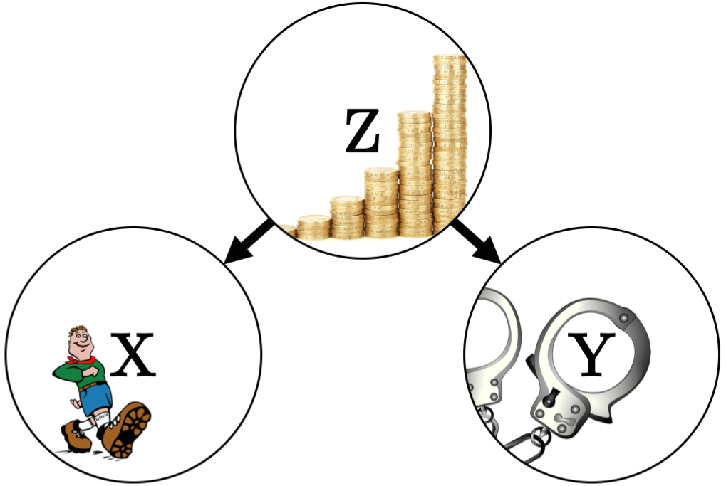
Nodes represent variables and edges (links) represent influence. Graphical models will be explained in further detail after the concept of conditional dependence is introduced.

Conditional dependence

If the equation presented in the previous section does not hold, we say that \(X\) and \(Y\) are conditionally dependent given \(\mathbf{Z}\). Intuitively, conditional dependence can be understood as a “competing” explanation by \(X\) and \(Y\), for a phenomenon \(\mathbf{Z}\). For example⁴, let \(X\) by a variable stating whether or not the sprinkler is on, let \(Y\) be a variable stating whether or not it is raining, and let \(Z\) be a variable stating whether or not the grass is wet. If we know that the grass is wet and we know that it is raining, then the probability that the sprinkler is on goes down. In other words, \(X\) has explained away \(Z\). The conditional dependence described here can be graphically represented as follows:

Note that, in this example, the (likely) marginal dependence between \(X\) and \(Y\) is ignored.

Graphical models

The simple networks in the previous two figures are examples of Bayesian networks, or directed graphical models, in which the edges have a direction assigned to them. In contrast, the edges in Markov networks, or undirected graphical models, are undirected. Both Bayesian and Markov networks can be used to visualize the factorization of the joint probability distribution \(J\) for a set of variables \(\mathbf{X}\).

Formally, a Bayesian network is a graphical model that encodes the conditional dependencies of a set of random variables in a directed acyclic graph (DAG). Under certain assumptions, which will be discussed in the next section, Bayesian networks can be used to capture causal structures⁵. The joint probability distribution of a set of variables in a Bayesian network is readily derived by considering the parents of each variable:

\[P(\mathbf{X}) = \prod_{X\in \mathbf{X}} P(X\mid Parents(X))\]

For example, from the conditional independence (scouting/delinquency) example, we know that \(P(X,Y,Z)\) factorizes as \(P(X\mid Z)P(Y\mid Z)P(Z)\). The Markov condition states that every variable \(X\) is conditionally independent of all other variables that are neither parents nor children of \(X\), given the parents of \(X\). The Markov condition generalizes to the criterion of d-separation for conditional independence, for which the full details are beyond the scope of this note (see Pearl⁶). It is sufficient to know, at this point, that d-separation is a set of rules that allow us to infer the conditional independencies from a DAG.

A Markov network captures the conditional (in)dependencies in an undirected graph. Inferring these dependencies is straightforward, using the following three Markov properties:

• Pairwise Markov property. Two non-adjacent variables are conditionally independent given all other variables.
• Local Markov property. A single variable is conditionally independent of all other variables given its neighbors. The local Markov property is the Markov network-equivalent of the Markov condition in Bayesian networks.
• Global Markov property. Two sets of variables \(\mathbf{X}\) and \(\mathbf{Y}\) are conditionally independent given a third set \(\mathbf{Z}\) if \(\mathbf{Z}\) is a separating subset.

The term “separating subset” can be understood in the intuitive sense, i.e. a set \(\mathbf{Z}\) is a separating set of \(\mathbf{X}\) and \(\mathbf{Y}\) if every path between \(\mathbf{X}\) and \(\mathbf{Y}\) passes through one or more variables in \(\mathbf{Z}\). For example, \(Z\) would be a separating subset of \(X\) and \(Y\) in the examples shown in previous sections, if both networks were undirected.

The Markov blanket \(MB(T)\) of the target variable \(T\) in a Bayesian network is the union of \(Children(T)\), \(Parents(T)\) and \(Parents(Children(T))\). In a Markov network, \(MB(T)\) is the set of nodes adjacent to \(T\). The Markov blanket has the useful property that for every set of variables \(\mathbf{X}\) with no members in \(MB(T)\), we know that \(\mathbf{X}\CI T \mid MB(T)\)⁶. This implies that the Markov blanket contains all necessary information to describe and predict \(T\), and any other variables are essentially redundant (feature selection!). Before further discussing how the Markov blanket can be used for feature selection, let’s check our assumptions for independence and causality first.

Assumptions for independence and causality

In his introduction to causal inference, Scheines⁷ explains the difference between the assumptions required to infer probabilistic independence and the assumptions required to infer causality, a theory developed by Spirtes et al.⁵. To understand these assumptions, we first introduce the concept of latent variables. In practice, there may be many unmeasured, or even unknown, variables. Such variables are called latent variables. Among the latent variables, there may be variables that induce relations between pairs of variables that do not correspond to causal relations between them⁸. These variables are called confounding factors. For example, had we not measured \(Z\) in the conditional independence example, then socio-economic background would have been a confounding factor for the observed relation between boy scout membership and delinquency.

If we are content with inferring conditional independence, then \(d\)-separation (for Bayesian networks) and the Markov properties (for Markov networks) provide us with all the necessary tools. To do so, though, we have to assume that the graphical model we obtained (through structure learning, discussed later) is an accurate representation of the true data, entailing the correct conditional independencies. Assuming that the conditional independencies encoded in the true distribution exactly equal the ones encoded in a DAG (via d-separation) is referred to as the faithfulness assumption. More specifically, the graph \(G\) is faithful to the joint distribution \(J\) of a set of variables \(\mathbf{X}\), meaning that every (conditional) independence in \(J\) can be derived from \(G\) using d-separation. The faithfulness assumptions also guarantees that the Markov blanket is unique⁹.

Inferring causality using Bayesian networks requires two additional assumptions, in addition to faithfulness. Firstly, causal sufficiency has to hold for the observed set of variables \(\mathbf{X}\), meaning that for every pair of variables in \(\mathbf{X}\), all common causes are also measured⁵. In other words, there should not be any confounding factors. Secondly, the Bayesian network \(G\) and joint probability distribution \(J\) needs to satisfy the causal Markov condition, which implies (1) that \(G\) contains an edge from \(X\) to \(Y\) if and only if \(X\) is a direct cause of \(Y\), and (2) that the set of variables \(\mathbf{X}\) giving rise to \(J\) is causally sufficient. Under the causal sufficiency and faithfulness assumptions, the Markov blanket in a Bayesian network contains the direct causes, direct effects and the direct causes of the direct effects of \(T\)².

As noted, the causal sufficiency assumption does not hold in many applications (including ours¹). It may not be feasible to measure all known parameters and even if we could, there is no guarantee that there are undiscovered parameters that may act as confounding factors. As a result, correlation does not imply causation in our data and we are very limited in our ability to draw conclusions regarding causality. The “next best” inference we can do is conditional (in)dependence, which is what we will focus on in the remaining sections. We will assume faithfulness, which is widely embraced⁷.

Feature Selection

The feature selection problem is defined as follows²: Given a \(N\) instances of a variable set \(\mathbf{X}\) drawn from the true distribution \(D\), a prediction algorithm \(C\) and a loss (model-performance) function \(L\), find the smallest subset of variables \(\mathbf{F} \subseteq \mathbf{X}\) such that \(\mathbf{F}\) minimizes the expected loss \(L(M,D)\), where \(M\) is the model trained using algorithm \(C\) and the feature set \(\mathbf{F}\). Informally, we aim to find the feature set \(\mathbf{F}\) that “optimally” characterizes the target variable \(T\)¹⁰.

In the previous section, we discussed the inference of conditional (in)dependence from Bayesian and Markov networks. The question is now: how do we utilize these tools for the purpose of feature selection and inference? Aliferis et al.² center their discussion on this topic around the Markov blanket. Indeed, given the fact that \(\mathbf{X}\CI T \mid MB(T)\), members of \(MB(T)\) intuitively seem like promising candidates for our maximally relevant and minimally redundant feature set.

The theoretical link between feature selection, Markov blankets and the definition of feature “relevance” is rigorously examined by Tsamardinos et al.¹¹, connecting their insights with the classical relevance definition by Kohavi and John¹². Tsamardinos et al. find, among other insights, that feature relevance is always dependent on the choice of prediction algorithm and model-performance metric. There is no universally applicable definition of relevancy for prediction. Moreover:

• Strongly relevant features, which contain information about \(T\) not found in any other features, are members of \(MB(T)\).
• Weakly relevant features, which contain information about \(T\) also found in other features, are not members of \(MB(T)\) but have an undirected path to \(T\)
• Irrelevant features, which contain no information about \(T\), are not members of \(T\) and have no undirected path to \(T\).

Assuming that a prediction method can learn the distribution \(P(T\mid MB(T))\) and the model-performance metric is such that the perfect estimation (optimal score of the metric) is attained with the smallest number of variables, then the Markov blanket of \(T\) is the optimal solution of the feature selection problem. We also know from the previous section that we can infer conditional (in)dependencies from the Markov blanket and the surrounding Bayesian/Markov network, providing insight into the relation structure.

Structure learning

So far, we have motivated the use of graphical models for feature selection by defining feature relevance and by introducing the Markov blanket. Moreover, we demonstrated the usefulness of graphical models for inference of conditional dependency and causality in previous sections. Throughout this discussion, we assumed the graphical model was known. In practice, we need to construct the model based on a set of observations.

To this end, structure learning for Markov and Bayesian networks has been the subject of extensive research in the last two decades ^{5 13 14}. The main objective is to learn the structure of the graphical model, based on a dataset of observations of the variables involved. Although some algorithms (see e.g. Koller and Mehran¹⁵) have been designed to only learn the Markov blanket, we focus on the more general problem of learning the structure between all variables. Several approaches to structure learning can be distinguished, including score-based structure learning ¹⁶, constraint-based structure learning⁵ and other methods (hybrid, restricted structural equation models, additive noise models).

Structure learning using score-based methods proceeds in two steps⁸. First, we define a scoring function that evaluates how well the model structure matches the observations (e.g. Likelihood score, Akaike’s Information Criterion (AIC) or Bayesian Information Criterion (BIC)). Second, we employ an algorithm that searches the combinatorial space of all possible model structures for the particular model structure that optimizes the scoring function. To move through the search space, we can add edges, delete edges, and, in the case of Bayesian networks, reverse the direction of edges. A number of search algorithms have been proposed, including:

• Stepwise methods for Markov networks start with an empty network and add edges (forward search) or start with a fully saturated network and delete edges (backward search) that result in the largest decrease in the scoring function.
• Hill-climbing methods start with an empty network, random network, or an initial network based on prior (expert) knowledge, and proceed to iteratively compute the score for all possible perturbations. The algorithm then picks the perturbation (i.e. edge addition/removal/reversal) that results in the largest score improvement. To avoid local optima, hill-climbing algorithms are often combined with random restarts and/or tabu lists. The latter prevents the algorithm from reversing the \(k\) most recent perturbations.

For a more detailed overview of structure learning, refer to the work by Koller and Friedman ⁸.

Conclusion

We have described causality, conditional independence, feature selection and Markov blankets. Theoretically, the Markov blanket of the variable to predict is a perfect solution for the feature selection problem, as outlined in the previous two section. In practice, however, (structure) learning the required graphical model of a set of random variables can be rather challenging. In my case, the random variables were all continuous and non-Gaussian, for which most existing structure learning methods (at the time) did not work. There have been some exciting developments in this area since then (using additive noise models, for example) which may prompt me to revisit this approach to feature selection in the future.

References

---